Automated Geometries

Very simple “shoebox”-like geometries can be built with electroacPy. These rectangular enclosures are built through their dimensions along the \(x\), \(y\) and \(z\) axes, and can include one or more sub-surfaces to represent radiating or impedance boundaries. This simple geometry builder is accessed through the shoebox class:

from electroacPy import gtb

# Lx = 0.340
# Ly = 0.6912
# Lz = 0.3862

box = gtb.shoebox(Lx,       # length along x axis (m)
                  Ly,       # length along y axis (m)
                  Lz        # length along z axis (m)
                  position  # optional, location of the box relative to the origin (default = "center")
                  minSize   # optional, minimum size of the mesh (default = 0.0057)
                  maxSize   # optional, maximum size of the mesh (default = 0.057)
                  )

box.build()  # build the shoebox in a "*.msh" file

This is technically all you need to create a simple shoebox mesh — see Fig. 55. However, if additional boundaries are needed, the shoebox class becomes more complex to understand. In the following, we go through the global/local coordinate system, faces reference and how to add boundaries.

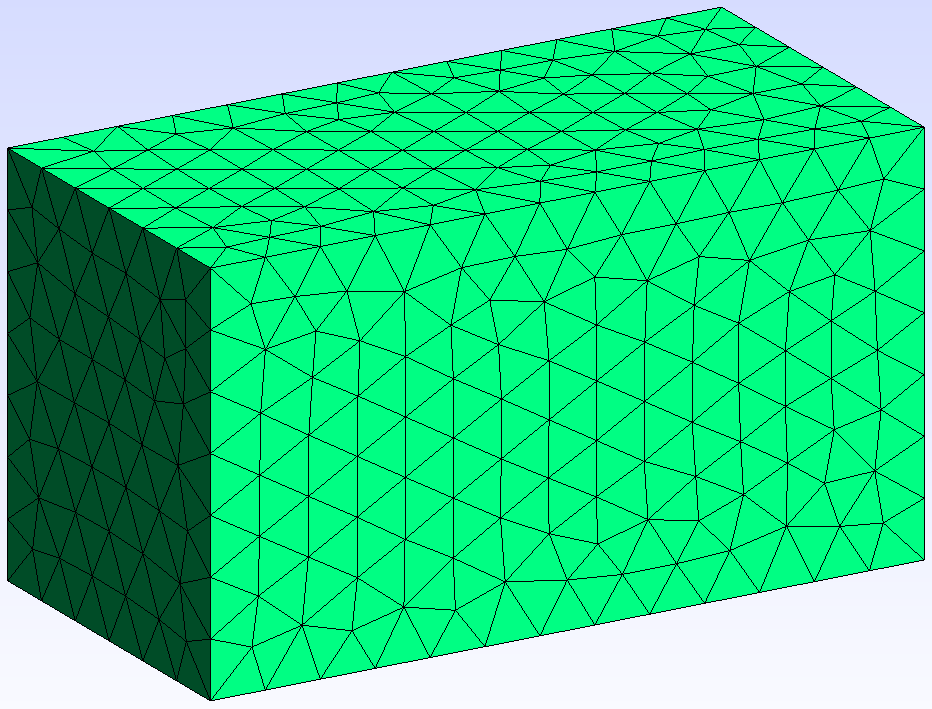
Fig. 55 Basic shoebox. With \(L_x = 0.340\), \(L_y = 0.6912\), \(L_z = 0.3862\).

Global and local coordinate system

First of all, the convention used in electroacPy to reference the faces of a box is shown in Fig. 56. Basically, the names of the six faces of a box are based on their outward normal direction in the global Cartesian coordinates. Each face is labeled according to the axis it is orthogonal to, with a sign indicating the direction of the outward normal.

Fig. 56 Face naming convention.

The “global coordinates” refer to the box positioning in space: if not specified, the box is centered at the origin of the global coordinates (\(x=0\), \(y=0\), \(z=0\)) as shown in Fig. 57-(a). If position="corner" is set as an input of .shoebox(), the origin is set at the back, lower-left corner of the box, as in Fig. 57-(b).

Fig. 57 (a) Default box configuration position="center". (b) Alternative corner position position="corner".

Local coordinates refers to the coordinates used when adding boundaries onto a face of the box. For example, a boundary created on the "+x" face will inherit the following local coordinates:

Fig. 58 (a) Local coordinates relative to the global Cartesian coordinates. (b) Local coordinates in the default configuration (i.e. local="center"). (c) Local coordinates in the corner configuration (i.e. local="corner"). See in the following sections for the local argument.

As you can see, depending on the local coordinates, the user can choose between center and corner positions. This choice is at the user’s discretion and is available for more convenience. At the moment, three boundary types can be added onto the mesh faces: circular, rectangular and polygonal geometries.

Circular boundaries

Fig. 59 (a) Centered local coordinates: local="center". (b) Corner-based local coordinates: local="corner".

Generally used for both drivers and ports, circular boundaries are created as follow:

box.addCircularBoundary(face,             # face on which the boundary is added
                        x,                # circle center along local x axis
                        y,                # circle center along local y axis
                        radius,           # radius of the circular boundary
                        physical_group,   # group reference for BEM simulation
                        mesh_size,        # mesh size on boundary
                        name=None,        # optional, name reference for BEM (not used by electroacpy, more useful to the user)
                        local="center")   # optional, positioning of local coordinates

The next example uses circular boundaries for the woofer, port and tweeter. The final geometry is shown in Fig. 60.

from electroacPy import gtb

# general dimensions
Lx = 0.3
Ly = 0.2
Lz = 0.4

# radius 
rt = 1.4e-2   # tweeter
rw = 6.1e-2   # woofer
rp = 2.5e-2   # port

# Creating the box
box = gtb.shoebox(Lx, Ly, Lz)
box.addCircularBoundary("x", 0.1, 0.190, rw, 
                        physical_group=1, name="woofer", local="corner")
box.addCircularBoundary("x", 0.048, 0.063, rp,
                        physical_group=2, name="port", local="corner")
box.addCircularBoundary("x", 0.1, 0.345, rt, 
                        physical_group=3, name="tweeter", local="corner")

# Saving the geometry
box.build("test_circular_b.msh")

Fig. 60 Shoebox enclosure with centered global coordinates and corner local coordinates.

Rectangular boundaries

Fig. 61 (a) Centered local coordinates: local="center". (b) Corner-based local coordinates: local="corner". The rectangle \(x\) and \(y\) position are given relative to its center of mass.

Rectangular boundaries will generally be used to describe ports or absorptive surfaces (e.g. carpets, wall panels, etc.). The following syntax is used:

box.addRectangularBoundary(face,             # face on which the boundary is added
                           x,                # rectangle's center of mass along local x axis
                           y,                # rectangle's center of mass along local y axis
                           lx,               # length along local x axis
                           ly,               # length along local y axis
                           physical_group,   # group reference for BEM simulation
                           mesh_size,        # mesh size on boundary
                           name=None,        # optional, name reference for BEM (not used by electroacpy, more useful to the user)
                           local="center")   # optional, positioning of local coordinates

Replacing the previous circular port by a rectangular one, the next bit of code gives Fig. 62.

# port dimension
lx_p = 0.08 
ly_p = 0.025

# Creating the box
# ...
# ...
# ...
box.addRectangularBoundary("x", 0.1, 0.063, lx_p, ly_p, 
                           physical_group=2, name="port", local="corner")

# Saving the geometry
box.build("test_rectangular_b.msh")

Fig. 62 Shoebox enclosure with rectangular port.

Polygonal boundaries

Fig. 63 (a) Centered local coordinates: local="center". (b) Corner-based local coordinates: local="corner". Notice that the coordinates must be given in the trigonometric direction — otherwise the mesh normals are inverted.

Polygonal boundaries are created as such:

box.addPolygonBoundary(face,            # face on which the boundary is put
                       X,               # list of local x coordinates for all points
                       Y,               # list of local y coordinates for all points
                       physical_group,  # group reference for BEM simulation
                       mesh_size,       # mesh size on boundary
                       name=None,       # optional, name reference for BEM (not used by electroacpy, more useful to the user) 
                       local="center")  # optional, positioning of local coordinates

Here, we describe the port as a split triangular configuration. As you can see in the next code snippet, multiple boundaries can be set in the same physical group. In that case, name will take the argument given in the first boundary declaration of that physical group. The mesh is shown in Fig. 64.

# Points coordinates
Xp1 = [0.025, 0.025, 0.075]  # port 1 - left-side of the enclosure
Yp1 = [0.06, 0.02, 0.02]

Xp2 = [0.175, 0.125, 0.175]  # port 2 - right-side of the enclosure
Yp2 = [0.06, 0.02, 0.02]

# Creating the box
# ...
# ...
# ...
box.addPolygonBoundary("x", Xp1, Yp1, 
                       physical_group=2, name="port", local="corner")
box.addPolygonBoundary("x", Xp2, Yp2, 
                       physical_group=2, local="corner")

# Saving the geometry
box.build("test_polygon_b.msh")

Fig. 64 Shoebox enclosure with triangular ports.