Point source

Acoustic monopoles are the simplest type of sound sources. They can be seen as single points in space, radiating sound waves in all directions. The mathematical expression of a monopole in the frequency domain can be written as follow:

\[ p(r) = jk\rho c Q \frac{e^{-jkr}}{4\pi r}, \]

where \(r\) is the distance from the monopole, \(k=\frac{2\pi f}{c}\) the wavenumber, \(\rho\) the density of propagation medium, \(c\) the speed of sound in said medium, and \(Q\) the volume velocity. Using a point source is practical when solving problems that are not specifically source related, such as the acoustic of a room.

Implementation

Monopole studies use the following syntax:

system.study_acousticPointSource("monopole",         # reference
                                 monopolePosition,   # list or numpy array
                                 acoustic_radiator,  # driver / enclosure objects
                                 meshPath=path,      # optional boundary mesh
                                 domain="interior")  # domain of simulation

where:

• monopolePosition can either be a numpy array of size (nSource, 3), or a vector of vectors (e.g. [[x1, y1, z1], [x2, y2, z2], ..., [xN, yN, zN]]),

• acoustic_radiator is defined in the same way as for .study_acousticBEM(). References to BEM need to be set even-though no mesh surface is radiating. Hence, ref2bem can be given arbitrarily,

• meshPath is optional: point source studies can be set with or without physical boundaries,

• domain is set to "exterior" or "interior", similarly to .study_acousticBEM().

Practical example

Let’s take a room of dimensions \(L_x=3.15\) m, \(L_y=5\) m and \(L_z=2.3\) m. We set a single point source in a corner, and evaluation point in the opposite position. In that case, we consider the walls to be fully reflective.

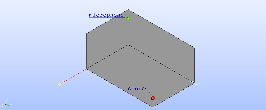
Fig. 28 Shoebox room, visualization done in Salome.

As usual, we start by importing libraries, setting the mesh path and initializing the system object:

import numpy as np
import electroacPy as ep
from electroacPy import gtb

#%% mesh data
room_mesh = "../geo/mesh/room.med"

#%% system initialization
frequency = np.arange(10, 200.25, 0.25)
sim = ep.loudspeakerSystem(frequency)

Now, the position of sources and evaluation points are written as vectors. The source has a unit velocity. In that case, ref2bem is set to 10 — even-though this value is not “used” directly as a reference to a mesh surface, the post-processing function will use it.

#%% source and microphone position
xSce = [2.85, 4.7, 0.3]
xMic_1 = [0.3, 0.3, 2] 
sim.lem_velocity("source", ref2bem=10)

Then, we create the study, add an evaluation and run simulations.

#%% study creation
sim.study_acousticPointSource("room", [xSce], "source",
                              meshPath=room_mesh, domain="interior")
sim.evaluation_fieldPoint("room", "corner_mic", [xMic_1])

#%% run
sim.run()

The acoustic pressure at the corner microphone — displayed in Fig. 29 — can be extracted as follow:

#%% extract data and plot
mic = sim.get_pMic("room", "corner_mic")
gtb.plot.FRF(frequency, mic, logx=False, xlim=(20, 200))

Fig. 29 Corner microphone pressure.

We can also compare the BEM simulation with the analytical solution of modes in a shoebox room:

\[f(n_x, n_y, n_z) = \frac{c}{2} \sqrt{\left(\frac{n_x}{L_x}\right)^2 + \left(\frac{n_y}{L_y}\right)^2 + \left(\frac{n_z}{L_z}\right)^2}\]

Fig. 30 Comparison between PSM/BEM acoustic pressure and analytical solution of room modes.

Finally, using sim.plot_pressureMesh("room") we display the pressure over the mesh:

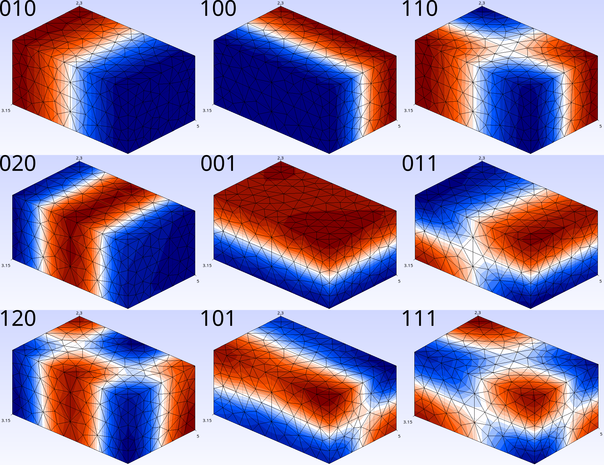
Fig. 31 Some room modes.