Boundary Element Modeler

ElectroacPy BEM modeler aims at automating the creation of bempp-cl studies: applying velocity to radiating elements, placement of evaluation points in 3D space, definition of the system based on boundary conditions, etc.

The BEM modeler is mostly focused on exterior acoustic radiation (e.g. a loudspeaker radiating in free-air), hence, a lot of functionality that you would find in commercial software are not available, such as interfaces between domains[1] or structural analysis. However, it is great for:

• diffraction studies,

• signal processing applied to loudspeaker array (beamforming, spherical harmonics, etc.),

• projection of measured/simulated acceleration data.

Fig. 14 Structure of the Boundary-Element Modeler.

.acoustic_study[]

The first computational step is to estimate the acoustic pressure on boundaries. The method .study_acousticBEM() is used for that effect. The inputs of .study_acousticBEM() are:

• name, study name, for reference purpose,

• meshPath, the path to simulated mesh,

• acoustic_radiator, the reference to enclosure and / or driver object that have been created beforehand,

• domain, relates to the type of study (i.e. "interior" or "exterior"), default is set to "exterior".

A few **kwargs are also available:

• tol, tolerance of the GMRES solver,

• boundary_conditions, a boundaryCondition object which defines infinite boundaries and surfaces impedance,

• direction, list of vector that add specific direction coefficients to the radiating surfaces, for example: [[0, 1, 0]] for a single driver radiating toward +y, or [[1, 0, 0], False, [1, 0, 0]] for three drivers, with two radiating toward +x and one with normal radiation direction. This last parameter is mostly useful when your radiators have a depth (e.g. a loudspeaker membrane not modeled as a flat surface).

In the following code, we define a free-field and a ground-reflected study.

import electroacPy as ep

#%% load data
system = ep.load("03_LEM_Recap")

#%% Define free-field study
system.study_acousticBEM("free-field", 
                         "../geo/mesh/studio_monitor.msh", 
                         ["ported_LF", "TW29", "sealed_MF"], 
                         domain="exterior")

#%% Define boundary conditions
from electroacPy.acousticSim.bem import boundaryConditions

bc = boundaryConditions()
bc.addInfiniteBoundary(normal="z", offset=-1)
system.study_acousticBEM("inf_ground", 
                        "../geo/mesh/studio_monitor.msh",
                        ["ported_LF", "TW29", "sealed_MF"], domain="exterior", 
                        boundary_conditions=bc)

#%% run boundary operators
system.run()

#%% save state
ep.save("04_BEM_setup", system)

The tweeter pressure on system’s boundaries is shown in Fig. 15. The mirrored mesh is due to the infinite boundary condition on the xy plane.

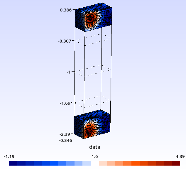
Fig. 15 Estimated pressure on boundary.

.evaluation[]

While computing the boundary pressure is the most computationally expensive step, it doesn’t provide a complete picture of the system. Information about the system’s radiated pressure (e.g. directivity, baffle diffraction, etc.) is obtained through the evaluation class, which efficiently automates the placement of observation points and visualization of results.

When an acoustic study is created, an evaluation object is automatically created. Hence, in regards to evaluations, the “only” functionality of loudspeakerSystem is to populate .evaluation["reference_study"] with observation setups. Six different observation types are available:

• .evaluation_polarRadiation(), get directivity information,

• .evaluation_pressureField(), pressure across rectangular screens,

• .evaluation_fieldPoint(), pressure at one (or more) user defined point,

• .evaluation_sphericalRadiation(), acoustic radiation within a sphere of radius \(r\),

• .evaluation_boundingBox(), pressure within a parallelepiped,

• .evaluation_plottingGrid(), import an external grid (must be a triangular mesh).

For our system, we define two polar radiations and two pressure-fields.

import electroacPy as ep

#%% load data
system = ep.load("04_BEM_setup")

#%% Define evaluations
system.evaluation_polarRadiation(["free-field", "inf_ground"], "polar_hor", 
                                 -180, 180, 5, on_axis="x", direction="y",
                                 radius=2, offset=[0, 0, 0.193])

system.evaluation_pressureField(["free-field", "inf_ground"], "field_ver", 
                                L1=3, L2=2, step=343/2500/6, 
                                plane="xz", offset=[-1.5, 0, -1])

system.evaluation_pressureField(["free-field", "inf_ground"], "field_hor", 
                                L1=3, L2=2, step=343/2500/6, 
                                plane="xy", offset=[-1.5, -1, 0.193])

system.evaluation_polarRadiation("free-field", "polar_ver", 
                                -180, 180, 5,  "x", "z", 
                                radius=2, offset=[0, 0, 0.193])

system.evaluation_polarRadiation("inf_ground", "polar_ver", 
                                0, 180, 5, "x", "z",
                                radius=2, offset=[0, 0, 0.193])

# system.plot_system("free-field")
# system.plot_system("inf_ground")

#%% run potential operators and plot results
system.run()
system.plot_results()

#%% save state
ep.save("05_evaluation_setup", system)

As you can see in this code, we use the .plot_system() function[2] — this will display the 3D placement of evaluation points and boundaries as shown by Fig. 16. You may also have noticed that the .run() command is used again: electroacPy automatically skips any boundary and potential evaluations already computed.

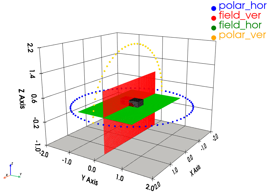
Fig. 16 System under study and related evaluations.

Acoustic results are displayed with .plot_results(), called from the system object. By default, all results will pop-up. It is possible to return specific results using the following arguments:

• study, select specific study or group of study,

• evaluation, select specific evaluation(s)

• radiatingElement, isolate radiating surfaces / elements

• bypass_xover, bypasses filters if crossovers are defined.

The following code displays Fig. 17.

system.plot_results(study="inf_ground", 
                    evaluation=["field_hor", "field_ver"],
                    radiatingElement=[1, 2])

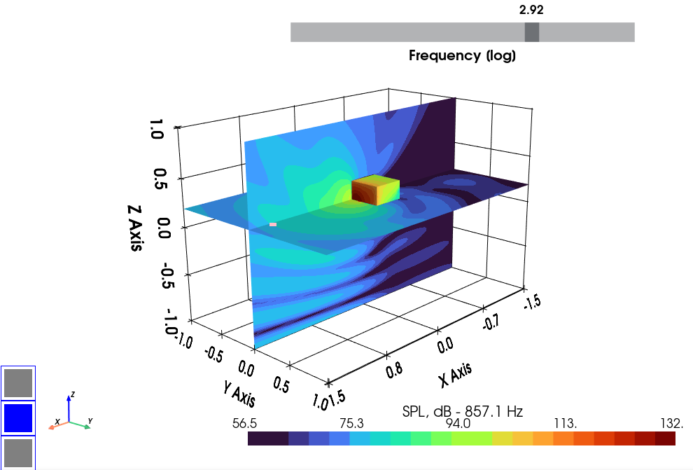
Fig. 17 Pressure-Field plotter.

When plotting a pressure field, a left click will return the frequency response function of the closest points. Fig. 18 is an example of this tool. The legend should display the (x, y, z) position of field point.

Fig. 18 Extraction of FRF from field point.

Polar responses are displayed using a Matplotlib viewer. It helps navigating through frequencies / angle with four sub-figures: SPL and normalized directivity, pressure and polar response — see Fig. 19.

Fig. 19 Directivity plotter. Horizontal radiation in free-field.

Note on imported grids

ElectroacPy can use external meshes as evaluation grids. The resulting plots are displayed through Gmsh by calling its api. This means that Gmsh should be installed on your system and accessible through your computer’s path. Depending on your OS, you’ll probably need to setup this yourself.

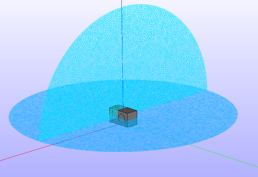
Fig. 20 Creating evaluation grids in Salome.

Adding a plotting grid to the evaluations can be done by simply pointing to the mesh path:

system.evaluation_plottingGrid("free-field", "hor_disc", 
                               "./geo/mesh/hor_disc_grid.msh")

Gmsh should open when calling the .plot_results() method. Two additional arguments can be passed:

• transformation, will plot the data with in different scales: spl, real, imag or phase. It is set to 'spl' by default,

• export_grid, if set to a path or file (e.g. "data_export.msh"), will save the visualization where told. This is particularly helpful when Gmsh cannot be called through the Python console.

Fig. 21 Custom grid through Gmsh viewer.

We won’t discuss the Gmsh viewer here as it is out of the scope of this documentation. However, you can access viewing options through the Tools/Options menu. From there you can change the color map and intervals, view names, visibility, and so on.

Code Summary

import electroacPy as ep
from electroacPy.acousticSim.bem import boundaryConditions

#%% load data
system = ep.load("03_LEM_Recap")

#%% Define free-field study
system.study_acousticBEM("free-field", 
                         "../geo/mesh/studio_monitor.msh",
                         ["ported_LF", "TW29", "sealed_MF"], domain="exterior")

#%% Define boundary conditions
bc = boundaryConditions()
bc.addInfiniteBoundary(normal="z", offset=-1)
system.study_acousticBEM("inf_ground", 
                        "../geo/mesh/studio_monitor.msh",
                        ["ported_LF", "TW29", "sealed_MF"], domain="exterior", 
                        boundary_conditions=bc)

#%% Define evaluations
system.evaluation_polarRadiation(["free-field", "inf_ground"], "polar_hor", 
                                 -180, 180, 5, "x", "y",
                                 radius=2, offset=[0, 0, 0.193])
system.evaluation_pressureField(["free-field", "inf_ground"], "field_ver", 
                                3, 2, 343/2500/6, "xz", offset=[-1.5, 0, -1])
system.evaluation_pressureField(["free-field", "inf_ground"], "field_hor", 
                                3, 2, 343/2500/6, "xy", 
                                offset=[-1.5, -1, 0.193])
system.evaluation_polarRadiation("free-field", "polar_ver", 
                                -180, 180, 5,  "x", "z", 
                                radius=2, offset=[0, 0, 0.193])
system.evaluation_polarRadiation("inf_ground", "polar_ver", 
                                0, 180, 5, "x", "z",
                                radius=2, offset=[0, 0, 0.193])

#%% run potential operators and plot results
system.run()
system.plot_results()

#%% save state
ep.save("06_acoustic_radiation", system)

---

[1]

It should be possible to implement it in bempp-cl.

[2]

Similar to Tkinter window, PyVista plotter will also stop execution of code.