Boundary Conditions

Boundaries are a key aspect of acoustic simulations. While a loudspeaker can generally be defined with infinitely rigid surfaces, some studies need to be given impedances and mirroring planes.

In that fashion, electroacPy provides the boundaryConditions class. While for now, it has only been used to create an infinite boundary (simulate the presence of a floor), it is possible to set impedance data on mesh surfaces.

Implementation

Boundary conditions should be passed as keyword arguments of the .study_acousticBEM() and .study_acousticPointSource() methods. A boundaryCondition object is created as follow:

from electroacPy.acousticSim.bem import boundaryConditions

bc = boundaryConditions(rho=1.22,  # optional
                        c=343)     # optional

At this stage, bc empty. Depending on the system’s boundaries, two methods are available:

• .addInfiniteBoundary(normal, offset),

• .addSurfaceImpedance(name, index, data_type, value).

It is important to note that infinite boundary conditions should only be used for exterior studies, as it creates a mirror of the system’s mesh.

Infinite boundaries

As an example, we can add an infinite boundary normal to \(z\) with no offset:

bc.addInfiniteBoundary(normal="z",  # axis normal to the boundary 
                       offset=0)    # offset of the boundary related to the normal axis

this gives the following system:

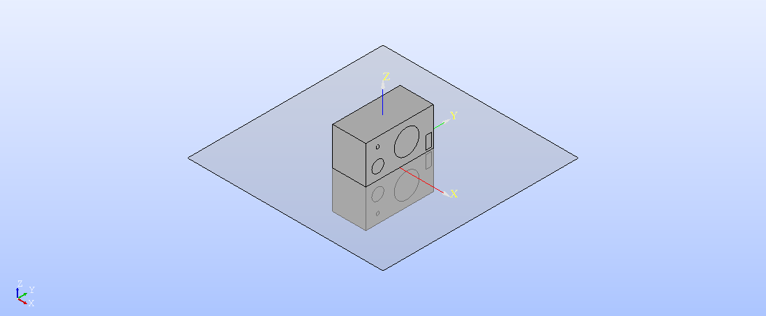
Fig. 32 Infinite boundary, with \(z\) normal to the mirror plane.

For now, electroacPy doesn’t provide automatic re-meshing functions in the case where surfaces between source and image are in contact. Hence it is better to leave a small offset (a few centimeters) to avoid source/image overlap.

In the case we want to have a 1 m offset:

bc.addInfiniteBoundary(normal="z",  # axis normal to the boundary 
                       offset=-1)    # offset of the boundary related to the normal axis

This sets an infinite boundary at 1 m below the source:

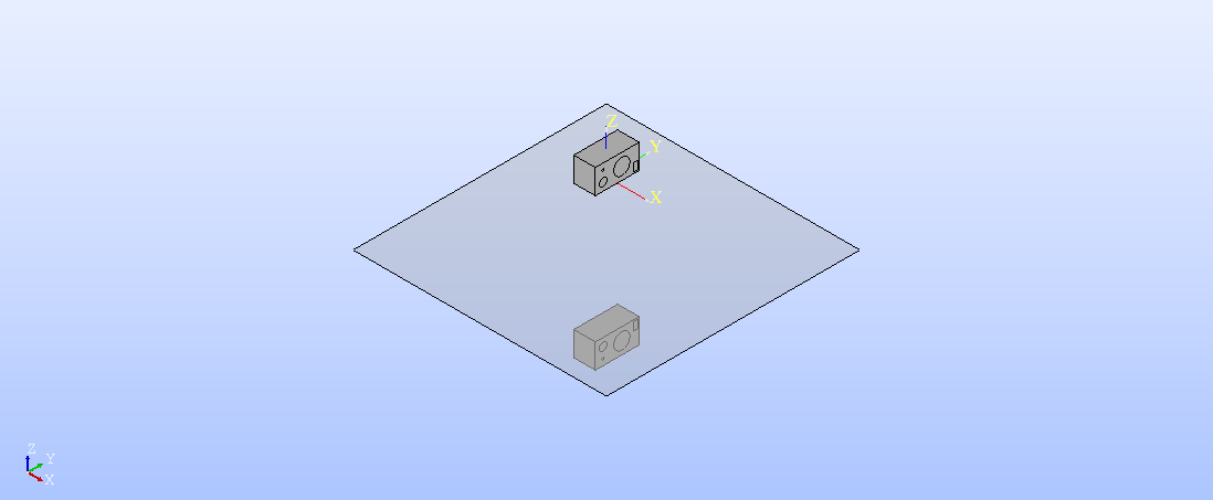
Fig. 33 Infinite boundary with an additional offset.

There is no hard-coded limit in the number of infinite boundaries a user can set. However, it is best not to exceed three infinite boundaries: one for each axis (\(x\), \(y\), \(z\)).

Surface Impedance

An impedance condition is created with this syntax:

bc.addSurfaceImpedance("name",          # reference 
                       index,           # BEM surface index
                       data_type,       # type of input data 
                       value,           # impedance data
                       frequency,       # optional, frequency range of "value"
                       targetFrequency, # optional, BEM frequency range (if "frequency" is different from the frequency axis given in the study object)
                       interpolation)   # optional, how to interpolate "frequency" on "targetFrequency)

A surface impedance is set over the physical groups listed in the index argument. Different “types” of impedance can be passed depending on data_type:

• "impedance": the specific impedance of the surface in \(\frac{Pa\times s}{m}\),

• "admittance": the inverse of specific impedance,

• "absorption": the absorption coefficient, between 0 and 1,

• "reflection": the reflection coefficient, between 0 and 1.

These data can either be given as single values or as frequency dependent variables. For its BEM computations, bempp-cl uses the normalized specific impedance \(Z_n = \frac{Z}{\rho c}\) — the normalization is done automatically.

Practical example

Because infinite boundaries were already explained in the .acoustic_study[] section, this example focuses on associating impedance to surfaces.

To keep some continuity in the documentation, we take the previous room acoustic simulation from the Point source chapter. We try to mitigate the first five modes, shown in Fig. 34.

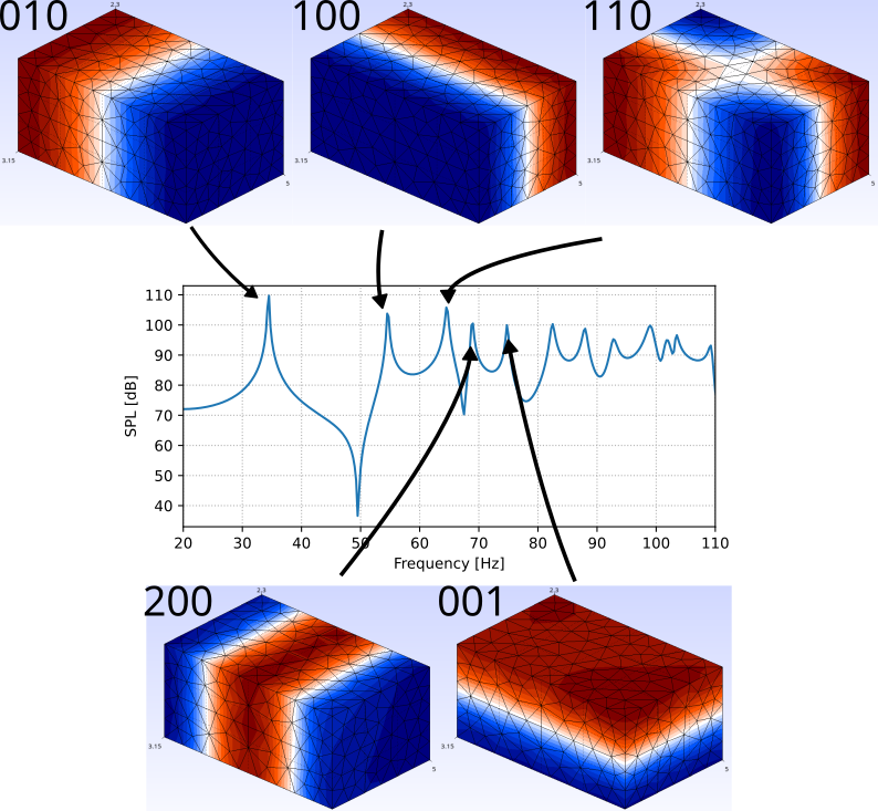
Fig. 34 Room response and first five modes.

Narrow-band absorber

In that room, the 34 Hz mode is relatively “far” (in term of frequency spacing) from the subsequent modes. To tackle it, we can use a narrow-band membrane absorber. Based on [KVorlander24], the impedance of a membrane absorber is written as:

\[Z = r_s + j\left( \omega M' - \frac{\rho c^2}{\omega d} \right),\]

with

• \(r_s\) the loss resistance, which can be expressed as a scalar multiple of \(Z_c\),

• \(M'\) the mass per surface area of the membrane,

• \(d\) the distance between the membrane and the back of the absorber.

The membrane mass \(M'\) is related to the target angular resonance (\(w_0=2\pi f_0\)):

\[M' = N \times \frac{\rho c}{w_0},\]

and \(d\) is given by:

\[d = \left( \frac{600}{f_0 \sqrt{M'}} \right)^2 \times 0.01.\]

If we set \(r_s=1 \times Z_c\) and \(N=5\), we get the impedance and absorption coefficients of Fig. 35:

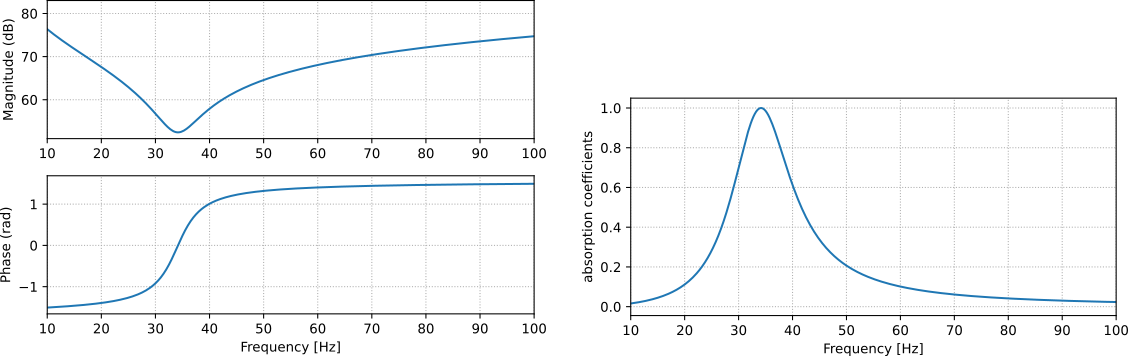
Fig. 35 Impedance (left) and absorption (right) of the 34 Hz narrow-band absorber.

Generally, the absorber is placed in a pressure extrema of the room — as shown in Fig. 36.

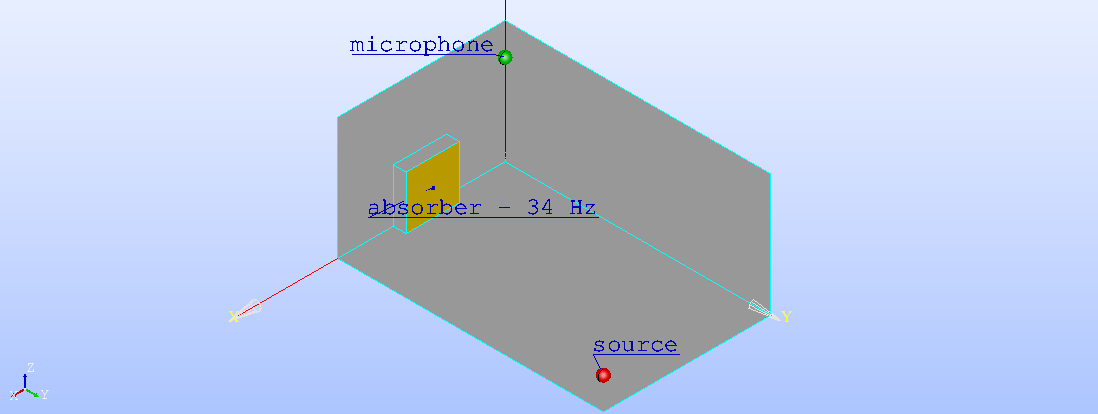
Fig. 36 Shoebox room with a membrane absorber.

To simplify a bit the code, we create a specific function for the absorber:

def resonance_absorber(frequency, f0, N, rs_factor, rho=1.22, c=343):
    """
    Create a resonance absorber

    Parameters
    ----------
    frequency : numpy array
        frequency range of the absorber.
    f0 : float
        resonant frequency.
    N : int
        Mass scaling factor.
    rs_factor : int or float
        Loss resistance factor, based on the air characteristic impedance. rs_factor=1 -> empty resonator (air) 
    rho : float, optional
        Air density. The default is 1.22.
    c : float, optional
        Speed of sound in air. The default is 343.

    Returns
    -------
    Z : numpy array
        Impedance response as function of frequency.

    """
    
    w   = 2 * np.pi * frequency
    w0  = 2 * np.pi * f0
    M   = N*rho*c/w0  # mass per m^2 of membrane
    d   = (600 / f0 / np.sqrt(M))**2 * 1e-2
    rs  = rs_factor * rho*c 
    Z = rs + 1j*(w*M - rho*c**2 / w / d)
    return Z

The simulation remains almost identical to the monopole study of the Point source chapter. The main differences are the input mesh and setting the boundary conditions in the .study_acousticPointSource() method.

#%% import functions
# ...
from electroacPy.acousticSim.bem import boundaryConditions

#%% mesh data
room_mesh   = "../geo/mesh/room_abs.msh"

#%% system initialization
# ...

#%% Define boundary conditions
Z = resonance_absorber(frequency, f0=34, N=5, rs=1)
bc = boundaryConditions()
bc.addSurfaceImpedance("absorber_34_Hz", 2, "impedance", Z)

#%% source and microphone position
# ...

#%% study creation
sim.study_acousticPointSource("room", [xSce], "source",
                              meshPath=room_mesh, domain="interior",
                              boundary_condition=bc)

Fig. 37 displays the resulting in-room response with a narrow-band absorber. Although the absorber significantly reduces the 34 Hz peak — which was the main target — slight alterations are noticeable at higher frequencies. These changes occur because the room’s effective volume decreases when the absorber is introduced.

Fig. 37 Comparison between the acoustic pressure with rigid walls and for a narrow-band absorber tuned at 34 Hz.

Wide-band absorber

Similar equations are employed to design a wide-band absorber centered at 64 Hz. For a simple resonator, achieving a wide bandwidth comes at the expense of a lower absorption coefficient. Regarding the placement of this absorber, the room’s mode shapes suggests that it is best to put it in a corner of the room. To do so, the absorber is divided into four smaller sections[1], as illustrated in Fig. 38. The new room configuration is meshed again.

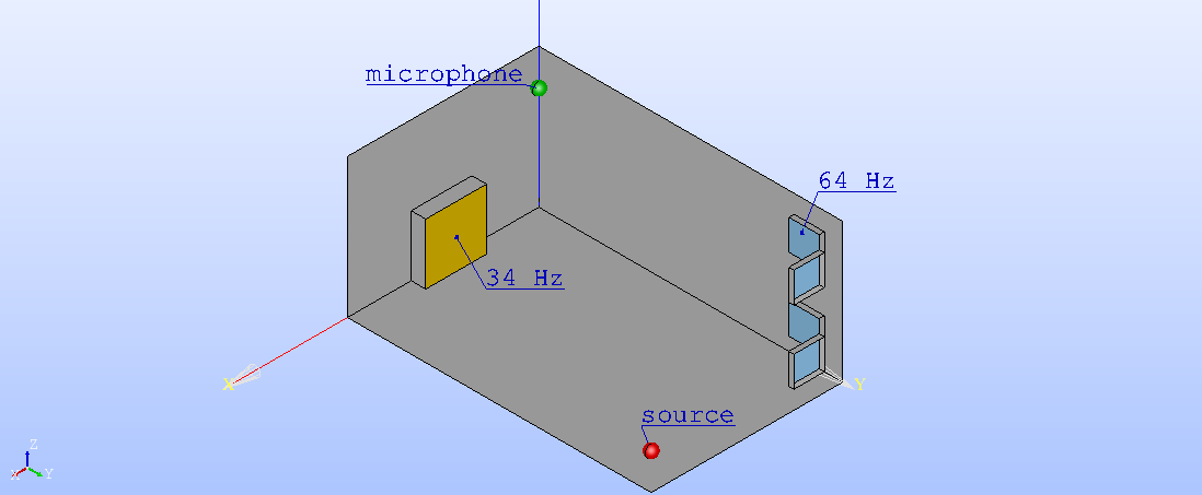
Fig. 38 Shoebox-room with 34 Hz and 64 Hz absorbers.

Using the previous resonance_absorber() function, we add another absorber to the simulation. Its impedance and absorption coefficients are displayed in Fig. 39:

Z2 = resonance_absorber(frequency, f0=64, N=5, rs=5)
bc.addSurfaceImpedance("absorber_64_Hz", 3, "impedance", Z2)

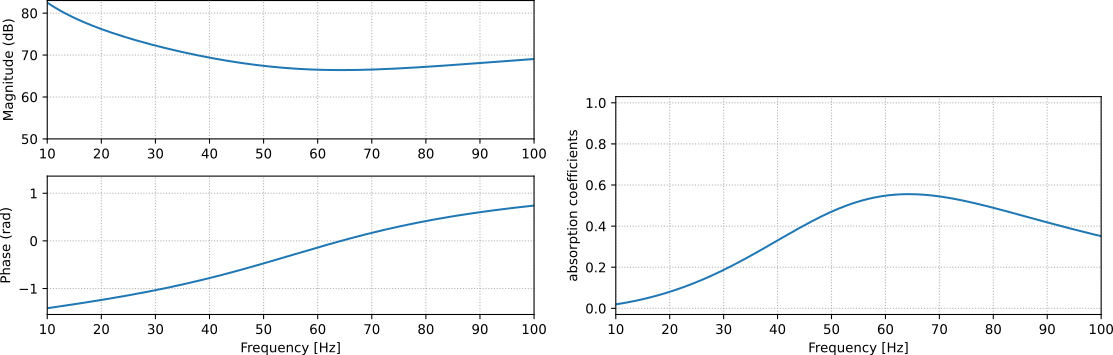
Fig. 39 Impedance (left) and absorption coefficient (right) of the large-band 64 Hz absorber.

In the end, we get the pressure response shown in Fig. 40.

Fig. 40 Frequency response comparison between 34 Hz absorber and the combination of 34 and 64 Hz absorbers.

---

[1]

To keep the same resonance and behavior, the depth of resonator should be changed. This was not done here for the sake of simplicity.