Evaluations

Studies are generally not complete without setting at least a few evaluation points in the observation domain. To do so, electroacPy provides functions to automate the placement of such points, as well as visualizations. Although a very brief introduction to evaluations has been provided in section .evaluation[], an in-depth explanation of this class is necessary. Hence, this part presents each available evaluation type in detail, from their initialization to the plotting tools.

Polar radiation

Polar evaluations focus on determining the directivity patterns of acoustic sources. This method is essential for understanding how sound radiates in different directions, providing insights into the polar distribution of acoustic energy.

Setup

Polar evaluations are defined as follow:

system.evaluation_polarRadiation("reference_study", # associated study    
                                 "evaluation_name", # evaluation label
                                 min_angle,         # minimum angle 
                                 max_angle,         # maximum angle
                                 step,              # angular step
                                 on_axis,           # 0-degree orientation '+-x', '+-y', '+-z'
                                 direction,         # angular direction '+-x', '+-y', '+-z'
                                 radius,            # optional, radius of polar plot
                                 offset,)           # optional, center offset

For example, a directivity setup with the following parameters gives Fig. 41:

minAngle  = -180
maxAngle  = 170
step      = 10
on_axis   = "x"
direction = "y"
radius    = 1.8

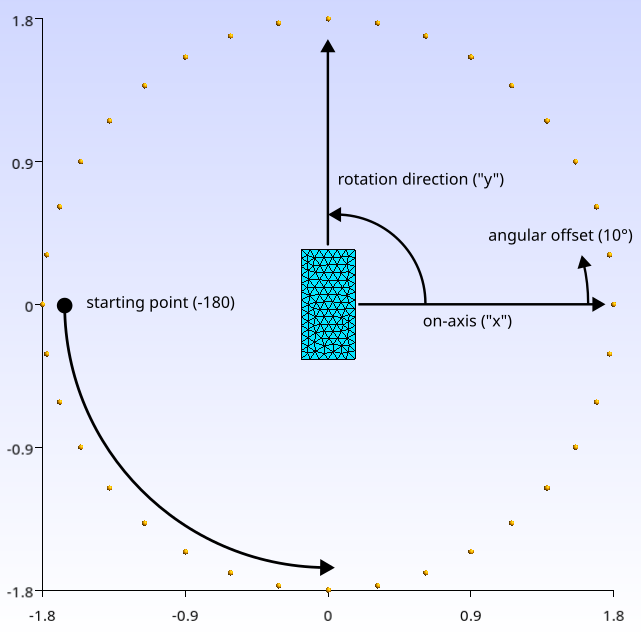
Fig. 41 Example of polar radiation settings. Top-down view of the monitor speaker.

Without setting an offset, the array is centered at (x=0, y=0, z=0). As shown in section .evaluation[], adding the argument offset=[0, 0, 0.193] moves the center of the array to the height of the woofer.

Visualization

Running the .plot_results() function displays the following matplotlib window:

Fig. 42 Visualization window for polar radiation evaluations.

This plot is interactive. Left-clicking on one of the left sub-plots will add the corresponding frequency response and polar plot to the top-right and bottom-right figures. Right-clicking will remove the most recently added frequency and polar response from the plot.

Spherical radiation

Spherical radiation evaluations compute the pressure distribution on a spherical surface surrounding the system. This results in a pseudo 3D-radiation-pattern.

Setup

Setting-up a spherical study is very simple:

system.evaluation_sphericalRadiation("reference_study", # associated study
                                     "evaluation_name", # evaluation label
                                     nMic,              # number of microphones on the sphere
                                     radius,            # sphere radius
                                     offset)            # center offset          

Similar to the polar radiation, radius and offset define the size and position of the evaluation sphere.

Fig. 43 Spherical array of evaluation points.

Visualization

Plotting results with a spherical evaluation displays a PyVista window:

Fig. 44 PyVista window for spherical evaluations.

Due to the limitations of PyVista, the slider widget needs to be written in a logarithmic way. The linear format of the current frequency is given in the figure title.

Pressure-field

Pressure-field evaluations calculate the acoustic pressure on a rectangular “screen” or plane. The resulting plot is a 2D slice of the observation domain.

Setup

Pressure-field observations are defined as follow:

system.evaluation_pressureField("reference_study", # reference study
                                "evaluation_name", # evaluation label
                                L1,                # length along the 1st dimension
                                L2,                # length along the 2nd dimension
                                step,              # spacing between evaluation points
                                plane,             # ex: "xy" with "x" 1st dimension and "y" 2nd dimension
                                offset)             

where

• L1 and L2 are the length along the first and second dimension (in metres),

• step is the target distance between two points,

• plane is a str variable that defines first and second dimensions (e.g. "xy", "-zx", etc.),

• offset will move the rectangular observation plane with the given cartesian coordinates.

These rectangular screens are built from their corner: without any offset, a plane described with the next parameters gives Fig. 45: the screen starts at x=0, y=0 and ends at x=L1, y=L2.

L1     = 2
L2     = 1
step   = 343 / 1000 / 6
plane  = "xy"
offset = [0, 0, 0]

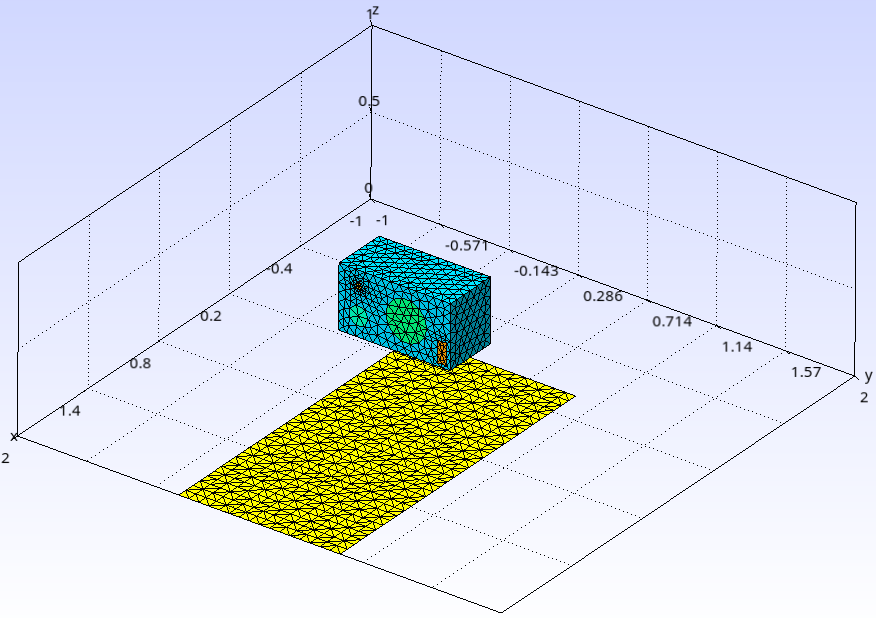
Fig. 45 Evaluation points for pressure-field grids.

Hence, if the screen is supposed to be placed in front of the loudspeaker, using offset = [0.2, -0.5, 0.193] moves it to the correct position, as shown in Fig. 46.

Fig. 46 Pressure-field with offset.

Visualization

For pressure-field visualizations, two backends are available: the default PyVista window or Gmsh. As usual, Gmsh must be set in the system path.

The default PyVista plotter gives Fig. 47:

Fig. 47 PyVista window for pressure-field visualizations.

To open the visualization with Gmsh, the argument pf2grid=True must be passed to the .plot_results() function:

system.plot_results(pf2grid=True)  # pressure-field to grid

The window in Fig. 48 is displayed.

Fig. 48 Gmsh window for pressure-field visualizations.

The advantage of using Gmsh is that it provides a lot of built-in options to change colormap, transformations, light position, mesh visibility and so on — see Fig. 49 for example.

Fig. 49 Some modifications of the visualization plot. We plot the real part of the pressure with system.plot_results(pf2grid=True, transformation="real").

Pressure-fields plotted as grids can be exported by either setting the additional export_grid argument, or by exporting grids through Gmsh. In the case that the grids are exported when plotting results, don’t forget to set the pf2grid=True argument:

system.plot_results(pf2grid=True, export_grid="file_name.msh")

Field-point

Field-point evaluations determine the acoustic pressure at specific user-defined Cartesian coordinates. This allows the user to compute the pressure at any available points.

Setup

Field point can be given as a matrix or as a numpy array of shape (nPoints, 3) of cartesian coordinates.

system.evaluation_fieldPoint("reference_study",  # reference study 
                             "evaluation_name",  # evaluation label
                             point_position)     # matrix or numpy array          

For example, the following code snippet results in Fig. 50.

# near-field microphone
mic_nf    = [[0.17 + 2e-2, 0.0725, 0.193], 
             [0.17+2e-2, 0.295, 0.092]]

# linear microphone array
mic_array = np.ones((20, 3))
mic_array[:, 0] *= np.linspace(0.17+0.15, 0.17+2, 20) 
mic_array[:, 1] *= 0.0725
mic_array[:, 2] *= 0.193

# add evaluation to study
system.evaluation_fieldPoint("free-field", "near-field", mic_nf)
system.evaluation_fieldPoint("free-field", "linear-array", mic_array)

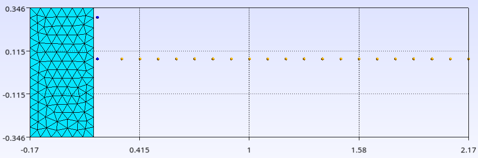
Fig. 50 Top-down view of a near-field (blue) and linear array (yellow) study.

Visualization

The default plot opens a matplotlib window.

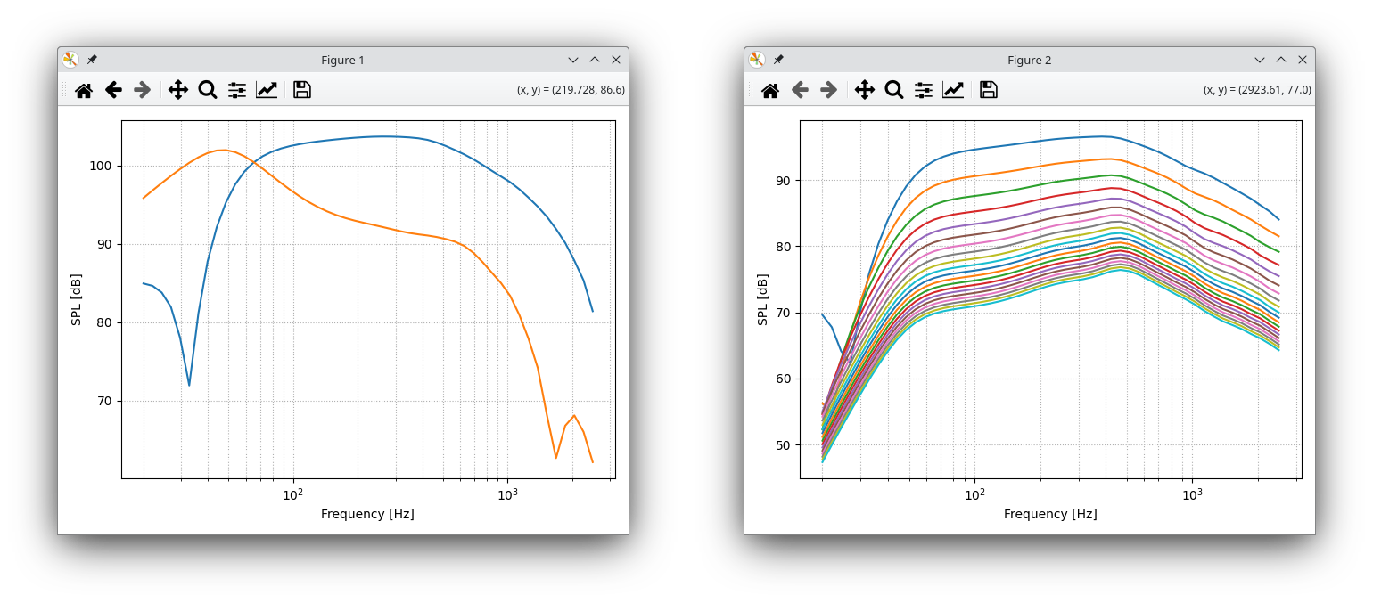
Fig. 51 Field-point display.

Usually, field-point studies are meant to be extracted from the system object with .get_pMic(). Afterward, the data can be displayed as desired.

As an illustration, we can plot the sound pressure level as a function of distance from the low-frequency driver:

import matplotlib.pyplot as plt
from electroacPy import gtb

# extract the pressure
p_array = system.get_pMic("free-field", "linear-array")

# get the index corresponding to 933 Hz
idx_f, freq = gtb.findInArray(system.frequency, 933) 

# Plot the attenuation
fig, ax = plt.subplots(figsize=(6, 3))
ax.plot(mic_array[:, 0] - 0.17, gtb.gain.SPL(p_array[idx_f, :]))
ax.grid(which="both", linestyle="dotted")
ax.set(xlabel="Distance from woofer [m]", ylabel="SPL [dB]")
plt.tight_layout()

Fig. 52 Attenuation of SPL with distance. This checks the -6 dB per doubling of distance.

Plotting-grids

Plotting-grids are user-made meshes on which the pressure is computed. Compatible formats are .msh and .med.

Setup

As long as the evaluation mesh is available, setting-up plotting-grids is very straightforward:

system.evaluation_plottingGrid("reference_study",  # reference study 
                               "evaluation_name",  # evaluation label
                               path_to_grid)       # path to evaluation mesh

In that fashion, we load two plotting-grids:

system.evaluation_plottingGrid("free-field", "hor_plane", "hor_plane.med")
system.evaluation_plottingGrid("free-field", "ver_plane", "ver_plane.med")

Using system.plot_system("free-field", "gmsh"), the total system is shown in Fig. 53.

Fig. 53 Importing two evaluation grids.

Visualization

For now, plotting-grids are only displayed through Gmsh. Depending on the input arguments, it is also possible to plot different visualizations or export data:

• transformation can be set to "real", "imag", "spl" or "phase": this changes the field’s value,

• export_grid saves the evaluation mesh in the given file (ex: "data_export.msh").

Fig. 54 Sound pressure distribution on imported grids.