Geometry import and meshing#
In the following sections, we demonstrate ElectroacPy’s capabilities using a three-way loudspeaker. The left sub-figure of Fig. 3 shows the system in its relatively complex CAD form: drivers are fully detailed, including the cone, basket, motor, etc., and the enclosure accounts for internal separations, port dimensions, and wall thickness. However, this level of detail is unnecessary for simple exterior-field studies, as many features will not significantly impact the acoustic radiation. Therefore, we simplify the system by retaining only the outer shell and representing each radiating element as flat surfaces — see the right sub-figure of Fig. 3. These significant simplifications should still provide valuable insights into acoustic radiation.
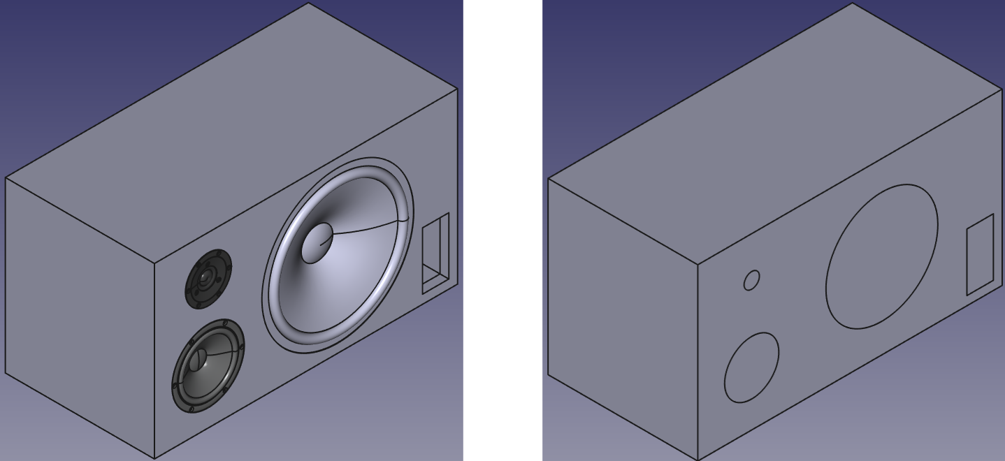
Fig. 3 CAD model (left) and simplified version for simulation (right).#
Mesh#
A mesh of the system is required for simulation with bempp. As noted in its documentation, mesh imports are handled with meshio. Compatible mesh formats are listed on its GitHub page[1]. To simplify the process of meshing geometries, ElectroacPy provides a small wrapper for the Gmsh API. This is what we’ll use for our study.
Once your geometry is exported as a .step file, you can create a CAD object with generalToolbox:
from electroacPy import gtb

cad = gtb.meshCAD("../geo/step_export/simulation_cad.step")
By default, the maximum mesh size corresponds to approximately 6 elements per wavelength at a frequency of 1 kHz, which equals 57 mm for a sound speed of 343 m/s. The minimum mesh size is ten times smaller: 5.7 mm. You can change these values by passing the minSize and maxSize arguments when importing a geometry:
cad = gtb.meshCAD("../geo/step_export/simulation_cad.step", minSize=343/2500/60,
maxSize=343/2500/6)
Next, surfaces must be grouped and referenced to set independent boundary or radiation conditions on separate surfaces. In our example, four radiating surfaces are considered:
cad.addSurfaceGroup("woofer", surface=[8], groupNumber=1)
cad.addSurfaceGroup("port", [10], 2)
cad.addSurfaceGroup("midrange", [9], 3)
cad.addSurfaceGroup("tweeter", [7], 4)
This code creates four surface groups numbered from 1 to 4, each referencing a different surface in the geometry. Surface indices can be retrieved from your CAD software. For example, FreeCAD displays the element index in the bottom-left corner when hovering over a surface, line, or point.
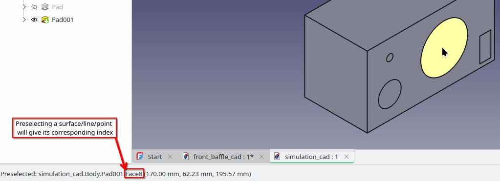
Fig. 4 Getting surface index.#
Once grouping of surfaces is done, run the mesh command. By default, it creates a 2D mesh under Gmsh’s .msh file format.
cad.mesh("../geo/mesh/studio_monitor")
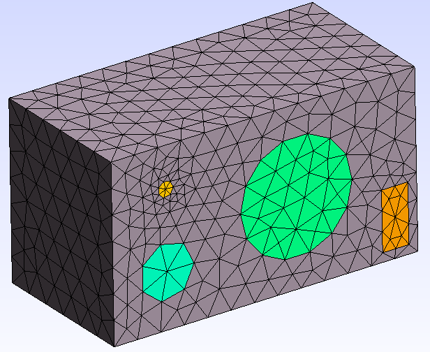
Fig. 5 Geometry meshed with a 1 kHz resolution.#
Of course, using a global mesh size can be restrictive. Therefore, it is possible to specify separate mesh sizes. In the following code, the global mesh size is set for 1 kHz, while the mesh is refined to 5 kHz over the tweeter and baffle surfaces.
#%% Set global size (1kHz)
lmax = 343/1e3/6
lmin = lmax/10
c
#%% import geo
cad = gtb.meshCAD("../geo/step_export/simulation_cad.step",
                  minSize=lmin, maxSize=lmax)

#%% group surfaces
cad.addSurfaceGroup("woofer", [8], 1)
cad.addSurfaceGroup("port", [10], 2)
cad.addSurfaceGroup("midrange", [9], 3)
cad.addSurfaceGroup("tweeter", [7], 4, meshSize=343/5e3/6)
cad.addSurfaceGroup("baffle", [3], 5, meshSize=343/5e3/6)
cad.mesh("../geo/mesh/studio_monitor_refined")
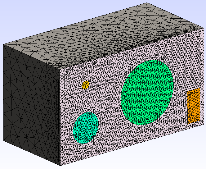
Fig. 6 Refined mesh.#
As you can see, although the smaller mesh was intended to be applied only to the tweeter and baffle, it is also present on the subwoofer, midrange, and port. This is a potential area for improvement in ElectroacPy’s automated API calls.
A final note: after creating surface groups, meshCAD will automatically regroup all remaining surfaces into a single group called “enclosure” — this ensures that all surfaces are properly loaded into bempp.
Automated Geometry#
Note
For more information, see Automated Geometries.
If you don’t have access to a CAD software, the mesh can be built directly in Python using Gmsh’s API. To simplify the process, gtb provides the shoebox class, allowing to quickly build simple loudspeaker geometries.
from electroacPy import gtb

# Enclosure dimensions
Lx = 0.340
Ly = 0.6912
Lz = 0.3862

# initialize a shoebox object
box = gtb.shoebox(Lx, Ly, Lz, position="corner")

# add boundaries corresponding to drivers and port
box.addCircularBoundary("x", 72.5e-3, 0, 127e-3, 1, name="woofer")
box.addRectangularBoundary("x", 295.6e-3, -107.6e-3, 60e-3, 131e-3, 2, name="port")
box.addCircularBoundary("x", -223.1e-3, -70.6e-3, 61.5e-3, 3, name="midrange")
box.addCircularBoundary("x", -223.1e-3, 101.2e-3, 17.4e-3, 4, name="tweeter")

# build and save the mesh in the ../geo folder
box.build("../geo/mesh/automated_mesh.msh")

Fig. 7 Mesh built with shoebox class.#