Post-processing

ElectroacPy provides some tools for crossover-network / filter design. These are considered “post-processing” as they are applied on computation results. It might not be the best term, but we’ll go with it for now.

.crossover[]

Crossovers/filters are initialized through the .filter_network() method. Input parameters are:

• name, network reference,

• ref2bem, which BEM elements should be filtered,

• ref2study, which study (or list of study) should receive the filter network.

Available filters are:

• lowpass and highpass, both under their “analog” form and as biquads,

• low-shelf, high-shelf,

• peaking eq,

• delay, gain and phase-flip,

• user-defined transfer functions.

In the code below, we define a crossover network using the available biquads:

from electroacPy import gtb
import electroacPy as ep
import numpy as np

#%% load data
system = ep.load("06_acoustic_radiation_refined")

#%% LF filter
system.filter_network("LF_xover", ref2bem=[1, 2], ref2study="free-field")
system.filter_addLowPassBQ("LF_xover", "lf1", 300, 0.5)

#%% MF Filter
system.filter_network("MF_xover", ref2bem=3, ref2study="free-field")
system.filter_addHighPassBQ("MF_xover", "hp1", 300, 0.5)
system.filter_addLowPassBQ("MF_xover", "lp1", 3500, 0.5)
system.filter_addGain("MF_xover", "db", -2)
system.filter_addPhaseFlip("MF_xover", "pi")

#%% HF Filter
system.filter_network("HF_xover", ref2bem=4, ref2study="free-field")
system.filter_addHighPassBQ("HF_xover", "hp1", 3500, 0.5, dBGain=-4)

Networks will automatically update the frequency response of previously computed studies. The .plot_results() method will display updated data. If you want to have a better look at each network response, you can either use the .plot_xovers() method, or extract the transfer function with .crossover["reference"].h — Fig. 22 is made using the following code:

#%% Transfer functions
H_lf = system.crossover["LF_xover"].h
H_mf = system.crossover["MF_xover"].h
H_hf = system.crossover["HF_xover"].h

gtb.plot.FRF(system.frequency, (H_lf, H_mf, H_hf, H_lf+H_mf+H_hf), 
             legend=("LF", "MF", "HF", "total"), transformation="dB",
             ylim=(-30, 10), xlim=(10, 10000), figsize=(6, 3),
             xticks=(10, 20, 50, 
                     100, 200, 500, 
                     1000, 2000, 5000, 10000),
             yticks=np.arange(-30, 12, 6))

Fig. 22 Crossover frequency-response.

It is also possible to extract and plot each individual pressure response using .get_pMic(), available through any loudspeaker system object. Here, we separate each acoustic radiator and look at the multiple contributions in Fig. 23.

# get pressure
p_lf   = system.get_pMic("free-field", "polar_hor", radiatingElement=1)
p_port = system.get_pMic("free-field", "polar_hor", radiatingElement=2)
p_mf   = system.get_pMic("free-field", "polar_hor", radiatingElement=3)
p_hf   = system.get_pMic("free-field", "polar_hor", radiatingElement=4)
p_tot  = system.get_pMic("free-field", "polar_hor")

# plot pressure response
gtb.plot.FRF(system.frequency, (p_lf[:, 73//2], 
                                p_port[:, 73//2],
                                p_mf[:, 73//2],
                                p_hf[:, 73//2],
                                p_tot[:, 73//2]), 
             ylabel="SPL [dB]",
             legend=("woofer", "port", "midrange", "tweeter", 
                     "total contribution"),
             xlim=(10, 10e3), ylim=(35, 80))

Fig. 23 Filtered loudspeaker response.

It is important to note that electroacPy’s crossover tools are considered as digital filters: interactions between speaker and supposed electrical components are not taken into account. In order to have a better understanding of the electrical behavior with passive components, it is either possible to use the circuitSolver class, or to export results to an external software for crossover design.

Export simulation data

For now, it is only possible to export directivity and impedance data. The following code extracts pressure and impedance with .export_directivity() and .export_impedance(). Results are then imported into VituixCAD as shown in Fig. 24. In the import window, you can notice that the “Minimum phase” box is checked: this helps reducing the comb-filtering coming from VituixCAD re-calculation of radiated pressure. Keep in mind that the overall radiation will be slightly off; you can un-check this box if you want a better estimation (although “noisier”).

The export syntax are:

# directivity
system.export_directivity(folder_path,      # path to export folder (mkdir if doesn't exists)
                          file_name,        # file prefix (angles are added to it)
                          study,            # study to export
                          evaluation,       # evaluation setup to export
                          radiatingElement, # radiating elements to export, optional
                          bypass_xover,     # if crossovers need to be bypassed, optional
                          frd)              # if True, uses *.frd extension, optional

# impedance
system.export_impedance(folder_path, # path to export folder (mkdir if doesn't exists)
                        file_name,   # file name
                        objName,     # driver object or enclosure object to export
                        zma)         # if True, uses *.zma extension, optional

In our case:

# export woofer data 

system.export_directivity("export/woofer", 
                           "polar_hor", "free-field", "polar_hor", 
                           radiatingElement=[1, 2], bypass_xover=True)
system.export_impedance("export_impedance", "ported_LF", "ported_LF")

# export midrange
system.export_directivity("export/midrange", 
                          "polar_hor", "free-field", "polar_hor", 
                          radiatingElement=3, bypass_xover=True)
system.export_impedance("export_impedance", "sealed_MF", "sealed_MF")

# export tweeter
system.export_directivity("export/tweeter", 
                           "polar_hor", "free-field", "polar_hor", 
                           radiatingElement=4, bypass_xover=True)
system.export_impedance("export_impedance", "TW29", "TW29")

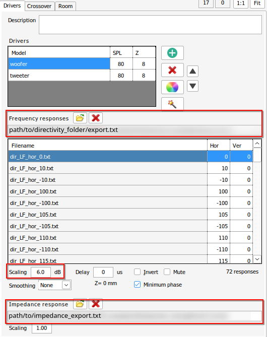
Fig. 24 Importing woofer simulation in VituixCAD. Because the directivity was estimated at 2 meters, a 6dB scaling is used to normalize it relative to 1 meter.

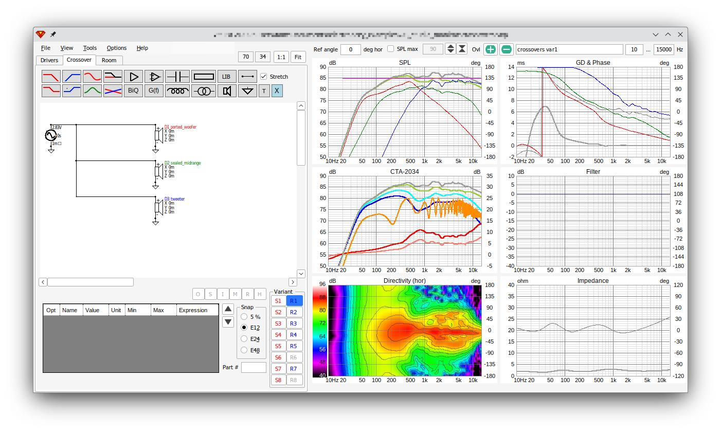
Fig. 25 Frequency response, directivity and impedance plot without crossovers.

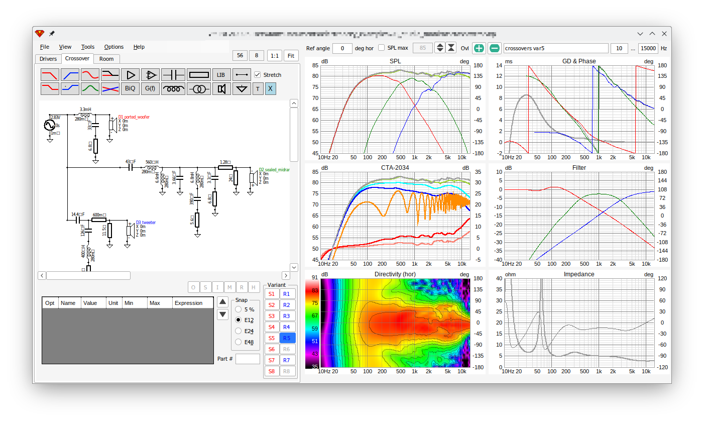
Fig. 26 Frequency response, directivity and impedance plot of system with crossovers.

If you’d rather use Xsim for your design, it is possible to add the frd=True and zma=True to the directivity and impedance export functions. By doing that, .export_directivity() and .export_impedance() use*.frd and *.zma extensions instead of *.txt.

# directivity export
system.export_directivity("export/woofer_FRD", 
                           "polar_hor", "free-field", "polar_hor", 
                           radiatingElement=[1, 2], bypass_xover=True, frd=True)

# impedance export
system.export_impedance("export_impedance_ZMA", "ported_LF", "ported_LF", zma=True)

Fig. 27 Crossover design with Xsim4.

As you’ll see in section Application example, it is possible re-create the above crossover using electroacPy’s own Modified Nodal Analysis (MNA) tool: circuitSolver.